Gráficos

Remuneração dos Servidores Públicos Federais

Autor

Afiliação

CGINF - Coordenação Geral de Informações Gerenciais

DIGID - Diretoria de Governança e Inteligência de dados

Resumo

Este tutorial aborda o cálculo e a visualização do Índice de Gini, uma medida estatística amplamente utilizada para avaliar a desigualdade na distribuição de renda em populações ou regiões.

1 Carregamento da base, limpeza e manipulação dos dados

Base bruta

# carregar a base de dados em excel e compilar todas as abas em um único arquivo


# Carregando as bibliotecas necessárias
library(readxl)
library(dplyr)
library(purrr)
library(tidyr)
library(ggplot2)
library(ggtext)
library(ggdist)
library(glue)
library(patchwork)
library(camcorder)
library(gt)
library(ggstatsplot)
library(plotly)
library(ggalt)

#gg_record(dir = "tidytuesday-temp", device = "png", width = 10, height = 8, units = "in", dpi = 320)

# Define o caminho do arquivo
file_path <- "data/BaseDados_EstudoDesigualdades.xlsx"

# Obtém os nomes de todas as abas no Excel
sheet_names <- excel_sheets(file_path)

# excluir abas que não serão utilizadas 
# aba FORA 

sheet_names <- sheet_names[!sheet_names %in% c("FORA")]

# Lê todas as abas e combina em uma única base usando purrr::map
BaseDados_Unica <- sheet_names %>%
  map_df(~ read_excel(file_path, sheet = .x) %>%
           mutate(sheet_name = .x)) # Adiciona o nome da aba como coluna (opcional)

# preencher valores NA na coluna escolaridade_cargo com "Não Informado"



# filtrar apenas campos que possuem servidores

df_gini <- BaseDados_Unica |> janitor::clean_names() |> 
  replace_na(list(escolaridade_cargo = "Sem informação")) |>
  rename( "2026" = ano_2026,  "2023"= mai_23 ) |>
  pivot_longer(`2023`:`2026`, names_to = "Ano", values_to = "remun") |>
  filter(qtd > 0) 

library(DT)

df_gini %>%
  datatable(
    rownames = FALSE,
    filter = "top",
    extensions = 'Buttons',
    options = list(
      pageLength = 5,
      scrollX = TRUE,
      dom = 'Bfrtip',  # B = Buttons, f = filter, r = processing, t = table, i = info, p = pagination
      buttons = c('copy', 'csv', 'excel')
    )
  ) %>%
  formatStyle(
    columns = names(df_gini), 
    target = "row",
    lineHeight = "12px",
    fontSize = "12px"
  )

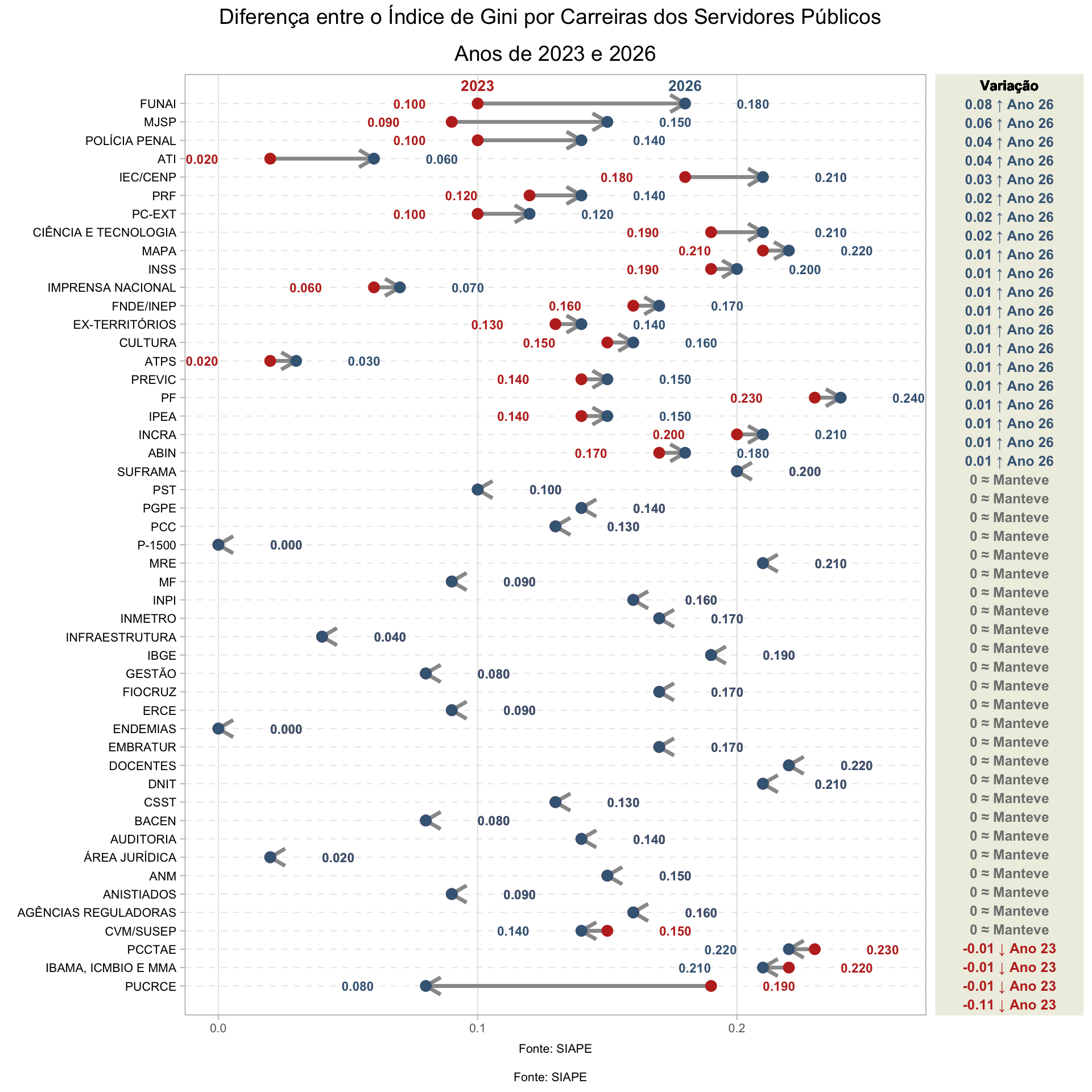
2 Gráfico dumbbell Carreiras

# Expandir a base de dados com base na quantidade de observações
df_expandido <- df_gini %>%
  uncount(qtd)

# Calculo do indice de gini por ano
df_gini_orgao <- df_expandido |> 
  #filter(Ano == "2023") |> 
  group_by(orgao_area, Ano) |>  
  summarise(
    total_remun = sum(remun, na.rm = TRUE),
    gini_index = ifelse(total_remun > 0, reldist::gini(remun), NA)
  ) |> 
  select(-total_remun) |>
  ungroup() |> 
  mutate(gini_index = round(gini_index, 2))
  


# pivotar wide 

df_gini_orgao_wide <- df_gini_orgao |> 
  pivot_wider(names_from = Ano, values_from = gini_index) |> 
  mutate(gap = `2026` - `2023`) |> 
  group_by(orgao_area) |>
  mutate(
    max=max(`2023`, `2026`)) |>
  ungroup() 
 

# Reordenando a variável orgao_area com base no gap em ordem decrescente

df_long_i <- df_gini_orgao_wide |> 
  arrange(gap) |> 
  mutate(labels=forcats::fct_reorder(orgao_area , gap)) |>
  ungroup()
 

df_long <- df_long_i %>% select(-c(orgao_area))%>% 
  pivot_longer(`2023`: `2026`, names_to = "name", values_to = "value") 

library(forcats)
library(scales)

nudge_value = 0.2

library(ggplot2)
library(dplyr)
library(tidyr)
library(scales)

# Assumindo que df_long_i já tenha as colunas "labels", "2023", "2026"

# Criando base para as setas
df_arrows <- df_long_i %>%
  mutate(
    x_start = `2023`,
    x_end = `2026`,
    y_pos = labels
  ) 

# Gráfico
p_main <- df_long %>%
  ggplot(aes(x = value, y = labels)) +
  
  # Adicionando setas entre 2023 e 2026
  geom_segment(data = df_arrows,
               aes(x = x_start, xend = x_end, y = y_pos, yend = y_pos),
               arrow = arrow(length = unit(0.4, "cm")),
               color = "gray60", linewidth = 1.2) +

  # Pontos
  geom_point(aes(color = name), size = 3) +

  # Rótulos com os valores
  geom_text(aes(label = label_number(accuracy = 0.001)(value), color = name),
            size = 3,
            fontface = "bold",
            nudge_x = if_else(df_long$value == df_long$max, 0.02, -0.02),
            hjust = if_else(df_long$value == df_long$max, 0, 1)) +
  
  # Rótulo do ano no final (caso deseje)
  geom_text(aes(label = name, color = name),
            data = df_long %>% filter(gap == max(gap)),
            nudge_y = 1,
            fontface = "bold",
            size = 3.5) +

  # Tema
  theme_light(base_size = 12) + 
  theme(legend.position = "none",
        axis.text.y = element_text(color = "black", size = 8),
        axis.text.x = element_text(color = "#666666", size = 8),
        axis.title = element_blank(),
        panel.grid.major.y = element_line(color = "gray90", linetype = "dashed"),
        panel.grid.minor = element_blank()) +
  
  # Título e fonte
  labs(
    title = "Anos de 2023 e 2026",
    caption = "Fonte: SIAPE"
  ) +

  # Cores
  scale_color_manual(values = c("#BF2F24", "#436685")) +

  # Limites
  coord_cartesian(ylim = c(0, 50))
# p_main

df_gap=
  df_long_i %>%  # note i am using df and not df_long
  mutate(
    label=fct_reorder(labels, abs(gap)), #order label by descending gaps
    
    gap_party_max = case_when(
  `2023` > `2026` ~ " ↓ Ano 23",
  `2023` == `2026` ~ " ≈ Manteve",
  TRUE ~ " ↑ Ano 26"
),
    
    # format gap values
    gap_label=
      paste0( round(gap, 2), gap_party_max) %>% 
      fct_inorder() #turns into factor to bake in the order
  )

#df_gap

p_gap=
  df_gap %>% 
  ggplot(aes(x=gap,y=labels)) +
  geom_text(aes(x=0, label=gap_label, color=gap_party_max),
            fontface="bold",
            size=3.25) +
  
  geom_text(aes(x=0, y=49.5), # 7 because that's the # of y-axis values
            label="Variação",
            nudge_y =.5, # match the nudge value of the main plot legend    
            fontface="bold",
            size=3.25) +
  
  theme_void() +
  coord_cartesian(xlim = c(-.05, 0.05), 
                  ylim=c(1,50) # needs to match main plot
  )+
  theme(
    plot.margin = margin(l=0, r=0, b=0, t=0), #otherwise it adds too much space
    panel.background = element_rect(fill="#EFEFE3", color="#EFEFE3"),
    legend.position = "none"
  )+
  scale_color_manual(values=c("#436685", "#BF2F24",  "grey50" )) 

#p_gap
p_main + p_gap + plot_layout(widths = c(1, 0.2)) +
  plot_annotation(
    title = "Diferença entre o Índice de Gini por Carreiras dos Servidores Públicos",
    caption = "Fonte: SIAPE"
  ) & 
  theme(plot.title = element_text(size = 14, hjust = 0.5),
        plot.caption = element_text(size = 8, hjust = 0.5))

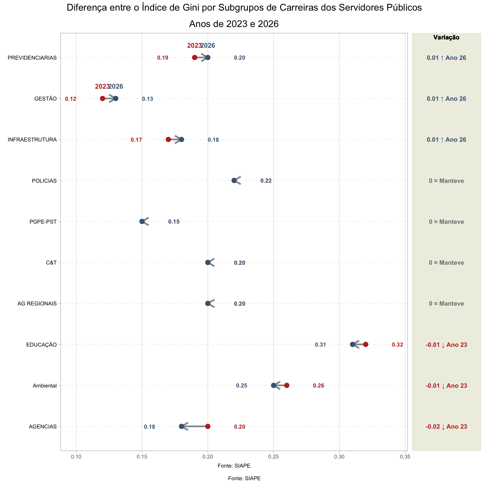
3 Gráfico dumbbell SubGrupos Carreiras

# Calculo do indice de gini por ano
df_gini_orgao <- df_expandido |> 
  #filter(Ano == "2023") |> 
  group_by(subgrupo, Ano) |>  
  summarise(
    total_remun = sum(remun, na.rm = TRUE),
    gini_index = ifelse(total_remun > 0, reldist::gini(remun), NA)
  ) |> 
  select(-total_remun) |>
  ungroup() |> 
  mutate(gini_index = round(gini_index, 2))
  


# pivotar wide 

df_gini_orgao_wide <- df_gini_orgao |> 
  pivot_wider(names_from = Ano, values_from = gini_index) |> 
  mutate(gap = `2026` - `2023`) |> 
  group_by(subgrupo) |>
  mutate(
    max=max(`2023`, `2026`)) |>
  ungroup() 
 

# Reordenando a variável orgao_area com base no gap em ordem decrescente

df_long_i <- df_gini_orgao_wide |> 
  arrange(gap) |> 
  mutate(labels=forcats::fct_reorder(subgrupo , gap)) |>
  ungroup()
 

df_long <- df_long_i %>% select(-c(subgrupo))%>% 
  pivot_longer(`2023`: `2026`, names_to = "name", values_to = "value") 

# Criando base para as setas
df_arrows <- df_long_i %>%
  mutate(
    x_start = `2023`,
    x_end = `2026`,
    y_pos = labels
  ) 

# Gráfico
p_main <- df_long %>%
  ggplot(aes(x = value, y = labels)) +
  
  # Adicionando setas entre 2023 e 2026
  geom_segment(data = df_arrows,
               aes(x = x_start, xend = x_end, y = y_pos, yend = y_pos),
               arrow = arrow(length = unit(0.4, "cm")),
               color = "gray60", linewidth = 1.2) +

  # Pontos
  geom_point(aes(color = name), size = 3) +

  # Rótulos com os valores
  geom_text(aes(label = label_number(accuracy = 0.01)(value), color = name),
            size = 3,
            fontface = "bold",
            nudge_x = if_else(df_long$value == df_long$max, 0.02, -0.02),
            hjust = if_else(df_long$value == df_long$max, 0, 1)) +
  
  # Rótulo do ano no final (caso deseje)
  geom_text(aes(label = name, color = name),
            data = df_long %>% filter(gap == max(gap)),
            nudge_y = 0.3,
            fontface = "bold",
            size = 3.5) +

  # Tema
  theme_light(base_size = 12) + 
  theme(legend.position = "none",
        axis.text.y = element_text(color = "black", size = 8),
        axis.text.x = element_text(color = "#666666", size = 8),
        axis.title = element_blank(),
        panel.grid.major.y = element_line(color = "gray90", linetype = "dashed"),
        panel.grid.minor = element_blank()) +
  
  # Título e fonte
  labs(
    title = "Anos de 2023 e 2026",
    caption = "Fonte: SIAPE"
  ) +

  # Cores
  scale_color_manual(values = c("#BF2F24", "#436685")) 

  # Limites
 # coord_cartesian(ylim = c(0, 50))
# p_main

df_gap=
  df_long_i %>%  # note i am using df and not df_long
  mutate(
    label=fct_reorder(labels, abs(gap)), #order label by descending gaps
    
    gap_party_max = case_when(
  `2023` > `2026` ~ " ↓ Ano 23",
  `2023` == `2026` ~ " ≈ Manteve",
  TRUE ~ " ↑ Ano 26"
),
    
    # format gap values
    gap_label=
      paste0( round(gap, 2), gap_party_max) %>% 
      fct_inorder() #turns into factor to bake in the order
  )

#df_gap

p_gap=
  df_gap %>% 
  ggplot(aes(x=gap,y=labels)) +
  geom_text(aes(x=0, label=gap_label, color=gap_party_max),
            fontface="bold",
            size=3.25) +
  
  geom_text(aes(x=0, y=10), # 7 because that's the # of y-axis values
            label="Variação",
            nudge_y =.5, # match the nudge value of the main plot legend    
            fontface="bold",
            size=3.25) +
  
  theme_void() +
  coord_cartesian(xlim = c(-.05, 0.05), 
                  ylim=c(1,10) # needs to match main plot
  )+
  theme(
    plot.margin = margin(l=0, r=0, b=0, t=0), #otherwise it adds too much space
    panel.background = element_rect(fill="#EFEFE3", color="#EFEFE3"),
    legend.position = "none"
  )+
  scale_color_manual(values=c("#436685", "#BF2F24",  "grey50" )) 

#p_gap
p_main + p_gap + plot_layout(widths = c(1, 0.2)) +
  plot_annotation(
    title = "Diferença entre o Índice de Gini por Subgrupos de Carreiras dos Servidores Públicos",
    caption = "Fonte: SIAPE"
  ) & 
  theme(plot.title = element_text(size = 14, hjust = 0.5),
        plot.caption = element_text(size = 8, hjust = 0.5))

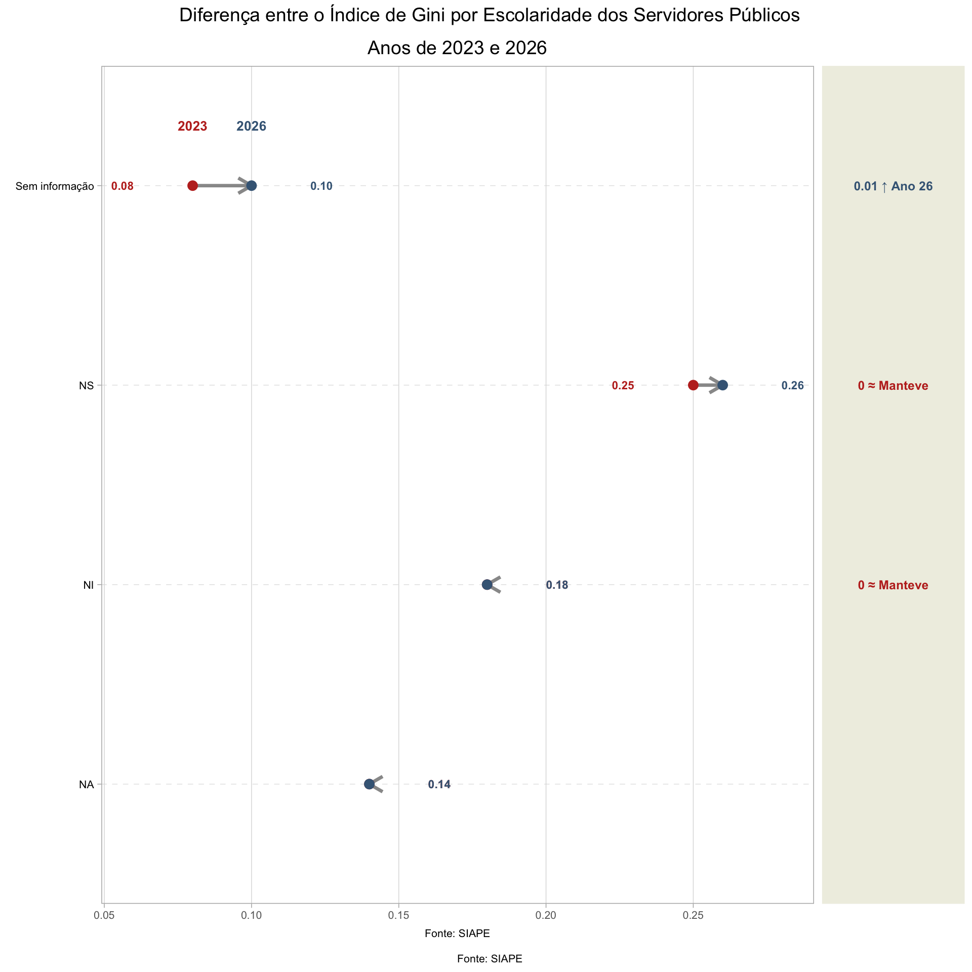
4 Gráfico dumbbell Escolaridade

# Calculo do indice de gini por ano
df_gini_orgao <- df_expandido |> 
  #filter(Ano == "2023") |> 
  group_by(escolaridade_cargo, Ano) |>  
  summarise(
    total_remun = sum(remun, na.rm = TRUE),
    gini_index = ifelse(total_remun > 0, reldist::gini(remun), NA)
  ) |> 
  select(-total_remun) |>
  ungroup() |> 
  mutate(gini_index = round(gini_index, 2))
  


# pivotar wide 

df_gini_orgao_wide <- df_gini_orgao |> 
  pivot_wider(names_from = Ano, values_from = gini_index) |> 
  mutate(gap = `2026` - `2023`) |> 
  group_by(escolaridade_cargo) |>
  mutate(
    max=max(`2023`, `2026`)) |>
  ungroup() 
 

# Reordenando a variável orgao_area com base no gap em ordem decrescente

df_long_i <- df_gini_orgao_wide |> 
  arrange(gap) |> 
  mutate(labels=forcats::fct_reorder(escolaridade_cargo , gap)) |>
  ungroup()
 

df_long <- df_long_i %>% select(-c(escolaridade_cargo))%>% 
  pivot_longer(`2023`: `2026`, names_to = "name", values_to = "value") 

# Criando base para as setas
df_arrows <- df_long_i %>%
  mutate(
    x_start = `2023`,
    x_end = `2026`,
    y_pos = labels
  ) 

# Gráfico
p_main <- df_long %>%
  ggplot(aes(x = value, y = labels)) +
  
  # Adicionando setas entre 2023 e 2026
  geom_segment(data = df_arrows,
               aes(x = x_start, xend = x_end, y = y_pos, yend = y_pos),
               arrow = arrow(length = unit(0.4, "cm")),
               color = "gray60", linewidth = 1.2) +

  # Pontos
  geom_point(aes(color = name), size = 3) +

  # Rótulos com os valores
  geom_text(aes(label = label_number(accuracy = 0.01)(value), color = name),
            size = 3,
            fontface = "bold",
            nudge_x = if_else(df_long$value == df_long$max, 0.02, -0.02),
            hjust = if_else(df_long$value == df_long$max, 0, 1)) +
  
  # Rótulo do ano no final (caso deseje)
  geom_text(aes(label = name, color = name),
            data = df_long %>% filter(gap == max(gap)),
            nudge_y = 0.3,
            fontface = "bold",
            size = 3.5) +

  # Tema
  theme_light(base_size = 12) + 
  theme(legend.position = "none",
        axis.text.y = element_text(color = "black", size = 8),
        axis.text.x = element_text(color = "#666666", size = 8),
        axis.title = element_blank(),
        panel.grid.major.y = element_line(color = "gray90", linetype = "dashed"),
        panel.grid.minor = element_blank()) +
  
  # Título e fonte
  labs(
    title = "Anos de 2023 e 2026",
    caption = "Fonte: SIAPE"
  ) +

  # Cores
  scale_color_manual(values = c("#BF2F24", "#436685")) 

  # Limites
 # coord_cartesian(ylim = c(0, 50))
# p_main

df_gap=
  df_long_i %>%  # note i am using df and not df_long
  mutate(
    label=fct_reorder(labels, abs(gap)), #order label by descending gaps
    
    gap_party_max = case_when(
  `2023` > `2026` ~ " ↓ Ano 23",
  `2023` == `2026` ~ " ≈ Manteve",
  TRUE ~ " ↑ Ano 26"
),
    
    # format gap values
    gap_label=
      paste0( round(gap, 2), gap_party_max) %>% 
      fct_inorder() #turns into factor to bake in the order
  )

#df_gap

p_gap=
  df_gap %>% 
  ggplot(aes(x=gap,y=labels)) +
  geom_text(aes(x=0, label=gap_label, color=gap_party_max),
            fontface="bold",
            size=3.25) +
  
  geom_text(aes(x=0, y=10), # 7 because that's the # of y-axis values
            label="Variação",
            nudge_y =.5, # match the nudge value of the main plot legend    
            fontface="bold",
            size=3.25) +
  
  theme_void() +
  coord_cartesian(xlim = c(-.05, 0.05), 
                  ylim=c(0,3) # needs to match main plot
  )+
  theme(
    plot.margin = margin(l=0, r=0, b=0, t=0), #otherwise it adds too much space
    panel.background = element_rect(fill="#EFEFE3", color="#EFEFE3"),
    legend.position = "none"
  )+
  scale_color_manual(values=c("#436685", "#BF2F24",  "grey50" )) 

#p_gap
p_main + p_gap + plot_layout(widths = c(1, 0.2)) +
  plot_annotation(
    title = "Diferença entre o Índice de Gini por Escolaridade dos Servidores Públicos",
    caption = "Fonte: SIAPE"
  ) & 
  theme(plot.title = element_text(size = 14, hjust = 0.5),
        plot.caption = element_text(size = 8, hjust = 0.5))